The hazard rate function, an introduction

The goal of this post is to introduce the concept of hazard rate function by modifying one of the postulates of the approximate Poisson process. The rate of changes in the modified process is the hazard rate function. When a “change” in the modified Poisson process means a termination of a system (be it manufactured or biological), the notion of the hazard rate function leads to the concept of survival models. We then discuss several important examples of survival probability models that are defined by the hazard rate function. These examples include the Weibull distribution, the Gompertz distribution and the model based on the Makeham’s law.

We consider an experiment in which the occurrences of a certain type of events are counted during a given time interval or on a given physical object. Suppose that we count the occurrences of events on the interval $(0,t)$ . We call the occurrence of the type of events in question a change. We assume the following three conditions:

The numbers of changes occurring in nonoverlapping intervals are independent.
The probability of two or more changes taking place in a sufficiently small interval is essentially zero.
The probability of exactly one change in the short interval $(t,t+\delta)$ is approximately $\lambda(t) \delta$ where $\delta$ is sufficiently small and $\lambda(t)$ is a nonnegative function of $t$ .

For the lack of a better name, throughout this post, we call the above process the counting process (*). The approximate Poisson process is defined by conditions 1 and 2 and the condition that the $\lambda(t)$ in condition 3 is a constant function. Thus the process we describe here is a more general process than the Poisson process.

Though the counting process indicated here can model the number of changes occurred in a physical object or a physical interval, we focus on the time aspect by considering the counting process as models for the number of changes occurred in a time interval where a change means “termination” or ‘failure” of a system under consideration. In many applications (e.g. in actuarial science and reliability engineering), the interest is on the time until termination or failure. Thus, the distribution for the time until failure is called a survival model. The rate of change function $\lambda(t)$ indicated in condition 3 is called the hazard rate function. It is also called the failure rate function in reliability engineering. In actuarial science, the hazard rate function is known as the force of mortality.

Two random variables naturally arise from the counting process (*). One is the discrete variable $N_t$ , defined as the number of changes in the time interval $(0,t)$ . The other is the continuous random variable $T$ , defined as the time until the occurrence of the first (or next) change.

Claim 1. Let $\displaystyle \Lambda(t)=\int_{0}^{t} \lambda(y) dy$ . Then $e^{-\Lambda(t)}$ is the probability that there is no change in the interval $(0,t)$ . That is, $\displaystyle P[N_t=0]=e^{-\Lambda(t)}$ .

We are interested in finding the probability of zero changes in the interval $(0,y+\delta)$ . By condition 1, the numbers of changes in the nonoverlapping intervals $(0,y)$ and $(y,y+\delta)$ are independent. Thus we have:

$\displaystyle P[N_{y+\delta}=0] \approx P[N_y=0] \times [1-\lambda(y) \delta] \ \ \ \ \ \ \ \ (a)$

Note that by condition 3, the probability of exactly one change in the small interval $(y,y+\delta)$ is $\lambda(y) \delta$ . Thus $[1-\lambda(y) \delta]$ is the probability of no change in the interval $(y,y+\delta)$ . Continuing with equation $(a)$ , we have the following derivation:

$\displaystyle \frac{P[N_{y+\delta}=0] - P[N_y=0]}{\delta} \approx -\lambda(y) P[N_y=0]$

$\displaystyle \frac{d}{dy} P[N_y=0]=-\lambda(y) P[N_y=0]$

$\displaystyle \frac{\frac{d}{dy} P[N_y=0]}{P[N_y=0]}=-\lambda(y)$

$\displaystyle \int_0^{t} \frac{\frac{d}{dy} P[N_y=0]}{P[N_y=0]} dy=-\int_0^{t} \lambda(y)dy$

Integrating the left hand side and using the boundary condition of $P[N_0=0]=1$ , we have:

$\displaystyle ln P[N_t=0]=-\int_0^{t} \lambda(y)dy$

$\displaystyle P[N_t=0]=e^{-\int_0^{t} \lambda(y)dy}$

Claim 2
As discussed above, let $T$ be the length of the interval that is required to observe the first change in the counting process (*). Then the following are the distribution function, survival function and pdf of $T$ :

$\displaystyle F_T(t)=\displaystyle 1-e^{-\int_0^t \lambda(y) dy}$
$\displaystyle S_T(t)=\displaystyle e^{-\int_0^t \lambda(y) dy}$
$\displaystyle f_T(t)=\displaystyle \lambda(t) e^{-\int_0^t \lambda(y) dy}$

In Claim 1, we derive the probability $P[N_y=0]$ for the discrete variable $N_y$ derived from the counting process (*). We now consider the continuous random variable $T$ . Note that $P[T > t]$ is the probability that the first change occurs after time $t$ . This means there is no change within the interval $(0,t)$ . Thus $S_T(t)=P[T > t]=P[N_t=0]=e^{-\int_0^t \lambda(y) dy}$ . The distribution function and density function can be derived accordingly.

Claim 3
The hazard rate function $\lambda(t)$ is equivalent to each of the following:

$\displaystyle \lambda(t)=\frac{f_T(t)}{1-F_T(t)}$
$\displaystyle \lambda(t)=\frac{-S_T^{'}(t)}{S_T(t)}$

Remark
Based on the condition 3 in the counting process (*), the $\lambda(t)$ is the rate of change in the counting process. Note that $\lambda(t) \delta$ is the probability of a change (e.g. a failure or a termination) in a small time interval of length $\delta$ . Thus the hazard rate function can be interpreted as the failure rate at time $t$ given that the life in question has survived to time $t$ . Claim 3 shows that the hazard rate function is the ratio of the density function and the survival function of the time until failure variable $T$ . Thus the hazard rate function $\lambda(t)$ is the conditional density of failure at time $t$ . It is the rate of failure at the next instant given that the life or system being studied has survived up to time $t$ .

It is interesting to note that the function $\Lambda(t)=\int_0^t \lambda(y) dy$ defined in claim 1 is called the cumulative hazard rate function. Thus the cumulative hazard rate function is an alternative way of representing the hazard rate function (see the discussion on Weibull distribution below).

Examples of Survival Models

Exponential Distribution
In many applications, especially those for biological organisms and mechanical systems that wear out over time, the hazard rate $\lambda(t)$ is an increasing function of $t$ . In other words, the older the life in question (the larger the $t$ ), the higher chance of failure at the next instant. For humans, the probability of a 85 years old dying in the next year is clearly higher than for a 20 years old. In a Poisson process, the rate of change $\lambda(t)=\lambda$ indicated in condition 3 is a constant. As a result, the time $T$ until the first change derived in claim 2 has an exponential distribution with parameter $\lambda$ . In terms of mortality study or reliability study of machines that wear out over time, this is not a realistic model. However, if the mortality or failure is caused by random external events, this could be an appropriate model.

Weibull Distribution
This distribution is an excellent model choice for describing the life of manufactured objects. It is defined by the following cumulative hazard rate function:

$\displaystyle \Lambda(t)=\biggl(\frac{t}{\beta}\biggr)^{\alpha}$ where $\alpha > 0$ and $\beta>0$

As a result, the hazard rate function, the density function and the survival function for the lifetime distribution are:

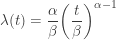
$\displaystyle \lambda(t)=\frac{\alpha}{\beta} \biggl(\frac{t}{\beta}\biggr)^{\alpha-1}$

$\displaystyle f_T(t)=\frac{\alpha}{\beta} \biggl(\frac{t}{\beta}\biggr)^{\alpha-1} \displaystyle e^{\displaystyle -\biggl[\frac{t}{\beta}\biggr]^{\alpha}}$

$\displaystyle S_T(t)=\displaystyle e^{\displaystyle -\biggl[\frac{t}{\beta}\biggr]^{\alpha}}$

The parameter $\alpha$ is the shape parameter and $\beta$ is the scale parameter. When $\alpha=1$ , the hazard rate becomes a constant and the Weibull distribution becomes an exponential distribution.

When the parameter $\alpha<1$ , the failure rate decreases over time. One interpretation is that most of the defective items fail early on in the life cycle. Once they they are removed from the population, failure rate decreases over time.

When the parameter $1<\alpha$ , the failure rate increases with time. This is a good candidate for a model to describe the lifetime of machines or systems that wear out over time.

The Gompertz Distribution
The Gompertz law states that the force of mortality or failure rate increases exponentially over time. It describe human mortality quite accurately. The following is the hazard rate function:

$\displaystyle \lambda(t)=\alpha e^{\beta t}$ where $\alpha>0$ and $\beta>0$ .

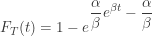
The following are the cumulative hazard rate function as well as the survival function, distribution function and the pdf of the lifetime distribution $T$ .

$\displaystyle \Lambda(t)=\int_0^t \alpha e^{\beta y} dy=\frac{\alpha}{\beta} e^{\beta t}-\frac{\alpha}{\beta}$

$\displaystyle S_T(t)=\displaystyle e^{\displaystyle \frac{\alpha}{\beta} e^{\beta t}-\frac{\alpha}{\beta}}$

$\displaystyle F_T(t)=\displaystyle 1-e^{\displaystyle \frac{\alpha}{\beta} e^{\beta t}-\frac{\alpha}{\beta}}$

$\displaystyle f_T(t)=\displaystyle \alpha e^{\beta t} \thinspace e^{\displaystyle \frac{\alpha}{\beta} e^{\beta t}-\frac{\alpha}{\beta}}$

Makeham’s Law
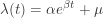
The Makeham’s Law states that the force of mortality is the Gompertz failure rate plus an age-indpendent component that accounts for external causes of mortality. The following is the hazard rate function:

$\displaystyle \lambda(t)=\alpha e^{\beta t}+\mu$ where $\alpha>0$ , $\beta>0$ and $\mu>0$ .

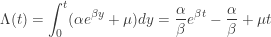
The following are the cumulative hazard rate function as well as the survival function, distribution function and the pdf of the lifetime distribution $T$ .

$\displaystyle \Lambda(t)=\int_0^t (\alpha e^{\beta y}+\mu) dy=\frac{\alpha}{\beta} e^{\beta t}-\frac{\alpha}{\beta}+\mu t$

$\displaystyle S_T(t)=\displaystyle e^{\displaystyle \frac{\alpha}{\beta} e^{\beta t}-\frac{\alpha}{\beta}+\mu t}$

$\displaystyle F_T(t)=\displaystyle 1-e^{\displaystyle \frac{\alpha}{\beta} e^{\beta t}-\frac{\alpha}{\beta}+\mu t}$

$\displaystyle f_T(t)=\biggl( \alpha e^{\beta t}+\mu t \biggr) \thinspace e^{\displaystyle \frac{\alpha}{\beta} e^{\beta t}-\frac{\alpha}{\beta}+\mu t}$

8 thoughts on “The hazard rate function, an introduction”

HC on October 29, 2011 at 9:35 am said:

Hi Dan:

I like you blog. Here is a question about the hazard rate, h(t), given F(t) = 1-exp(-lambda*t) for t in (0, t_max) and given that F(t) jumps up to 1 at t = t_max.

When F(t) is continuous in (0, inf), h(t)=f(t)/(1-F(t) is always fixed at lambda. But does h(t) remain fixed at lambda if F(t) is discontinuous at t = t_max, as mentioned above.

HC

Reply ↓
Dan Ma on November 2, 2011 at 11:18 pm said:

Hi, HC

Thanks for your comment and question. The response to your question can be found in the following post.

Defining Hazard Rate at a Point Mass

Dan

Reply ↓
HC on November 10, 2011 at 12:45 pm said:

Hi, Dan:
Thank you very much for your clarification. It is very helpful. Can I therefore assert the following:

#1. Given F(t) = 1-exp(-lambda*t) for t in (0, inf), hazard rate h(t) = lambda for t in (0, inf).

#2. Given F(t) = 1-exp(-lambda*t) for t in (0, t_max) and given that F(t) jumps up to 1 at t = t_max, hazard rate h(t) = lambda for t in (0, t_max) or h(t) = 1 at t = t_max.

Can you verify these assertions? Thanks.

Reply ↓
- Dan Ma on November 10, 2011 at 7:55 pm said:
  
  Yes, what you stated is exactly what the blog post is saying.
  
  Reply ↓
HC on November 10, 2011 at 2:40 pm said:

Hi, Dan,

Another question:
You said that h(t) = 1 at the point mass of t = t_max. But h(t) = P(t) / P(T > t) at t = t_max. Look, the survival function P(T > t) must be zero at t = t_max. Therefore, can we say that h(t) goes to infinity at t = t_max?

That is, my thoughts suggest that at t in (0, t_max), h(t) = lambda, but h(t) should shoot up to infinity at t = t_max. Can you comment on this, in addition to the earlier posted questions? Thanks.

HC

Reply ↓
- Dan Ma on November 10, 2011 at 8:00 pm said:
  
  I understand your confusion. I was confused for a little while too. At a point mass $T=t$ , $\displaystyle h(t)=\frac{P(T=t)}{P(T \ge t)}$ and not $\displaystyle h(t)=\frac{P(T=t)}{P(T > t)}$ . When the cdf has a jump, you cannot use $P(T > t)$ for the survival function at the jump.
  
  You can also keep in mind that at a point mass, the hazard rate is a conditional probability of dying at that point given the life survives up to that point. If the point mass is the last point in the life span, then this conditional probability has to be 1 (it is certain that the life will terminate).
  
  In the continuous case, the hazard rate is only a rate of termination and not necessarily a probability. In the discrete case, the hazard rate is a probability (a conditional probability: a probability of termination given survival up to that point). This is all explained in the blog post Defining Hazard Rate at a Point Mass.
  
  Hope this helps.
  
  Reply ↓
hwanlinHC on November 11, 2011 at 9:15 am said:

Hi, Dan,
Thank you very much.
HC

Reply ↓
Tariq on July 19, 2015 at 10:03 pm said:

What would be the numerical value of u in th efinal equation

Reply ↓