Mixed distributions arise naturally in many applications. In this post and in the next several posts we discuss several examples of mixed distributions based on insurance concepts. We then illustrate the calculation using the exponential distribution as the model for the random loss.
The support of a random variable  is the subset
  of the real numbers on which the probability mass function (if is discrete) or the probability density function (if is continuous) is positive. If is any continuous random variable,
 ![P[X=a]=0](https://s0.wp.com/latex.php?latex=P%5BX%3Da%5D%3D0&bg=ffffff&fg=333333&s=-1&c=20201002) for any
for any  . On the other hand, if is any discrete random variable,
 ![P[X=a] > 0](https://s0.wp.com/latex.php?latex=P%5BX%3Da%5D+%3E+0&bg=ffffff&fg=333333&s=-1&c=20201002) for any . In other words, a discrete distribution consists of a finite or countably infinite number of probability masses (or point masses) while continuous distributions have no point masses. This is one distinguishing characteristic between continuous random variables and discrete random variables. Mixed distributions (or mixed random variables) are nether continuous nor discrete. This means if has a mixed distribution, has at least one probability mass (i.e.
for any . In other words, a discrete distribution consists of a finite or countably infinite number of probability masses (or point masses) while continuous distributions have no point masses. This is one distinguishing characteristic between continuous random variables and discrete random variables. Mixed distributions (or mixed random variables) are nether continuous nor discrete. This means if has a mixed distribution, has at least one probability mass (i.e. ![P[X=a]>0](https://s0.wp.com/latex.php?latex=P%5BX%3Da%5D%3E0&bg=ffffff&fg=333333&s=-1&c=20201002) for at least one ) and it is also true that there is some interval
for at least one ) and it is also true that there is some interval  such that
 ![P[X=c]=0](https://s0.wp.com/latex.php?latex=P%5BX%3Dc%5D%3D0&bg=ffffff&fg=333333&s=-1&c=20201002) for all
for all  .
.
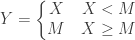
Let’s consider one insurance example of a mixed distribution. Let be the size (in dollar amount) of a random loss for an insurance contract. Suppose that the insurance contract has a policy maximum of  . For the purpose of this discussion, we assume that is a continuous random variable. We also assume that
 ![P[X>M]>0](https://s0.wp.com/latex.php?latex=P%5BX%3EM%5D%3E0&bg=ffffff&fg=333333&s=-1&c=20201002) . If the random loss is less than , the insurer pays the entire random loss amount. If the random loss exceeds , the insurance payout is capped at . Let
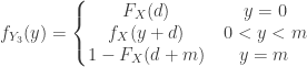
. If the random loss is less than , the insurer pays the entire random loss amount. If the random loss exceeds , the insurance payout is capped at . Let  be the “per loss” amount payable by the insurer. Then is determined by the following rule:
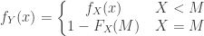
Since the random loss has a continuous distribution,  , the distribution function of , is a continuous function. Then the insurance payout has a mixed distribution. The distribution of has a probability mass (point mass) at
  and the distribution is continuous on the interval
  . The cumulative distribution function
  of is a step function with a jump at . The following is
  :
:

Since the right tail  is positive, has a jump at . The size of the jump is
  , which is the size of the point mass at
  . The density function of is a hybrid one:
The following derives the mean and the higher moments of the insurance payout.
![\displaystyle E[Y]=\int_0^{M} x \thinspace f_X(x) \thinspace dx + M \thinspace [1-F_X(M)]](https://s0.wp.com/latex.php?latex=%5Cdisplaystyle+E%5BY%5D%3D%5Cint_0%5E%7BM%7D+x+%5Cthinspace+f_X%28x%29+%5Cthinspace+dx+%2B+M+%5Cthinspace+%5B1-F_X%28M%29%5D&bg=ffffff&fg=333333&s=-1&c=20201002)
![\displaystyle E[Y^n]=\int_0^{M} x^n \thinspace f_X(x) \thinspace dx + M^n \thinspace [1-F_X(M)]](https://s0.wp.com/latex.php?latex=%5Cdisplaystyle+E%5BY%5En%5D%3D%5Cint_0%5E%7BM%7D+x%5En+%5Cthinspace+f_X%28x%29+%5Cthinspace+dx+%2B+M%5En+%5Cthinspace+%5B1-F_X%28M%29%5D&bg=ffffff&fg=333333&s=-1&c=20201002) for all integers
for all integers 
Consequently, the following computes the variance of the insurance payout :
![\displaystyle Var[Y]=E[Y^2]-\biggl(E[Y]\biggr)^2](https://s0.wp.com/latex.php?latex=%5Cdisplaystyle+Var%5BY%5D%3DE%5BY%5E2%5D-%5Cbiggl%28E%5BY%5D%5Cbiggr%29%5E2&bg=ffffff&fg=333333&s=-1&c=20201002)
Example of Calculation
Suppose we have an insurance contract with a policy maximum . Furthermore, the random loss amount in the insurance contract has an exponential distribution with parameter  . Then
  . The distribution function of the insurance payout is:

In the distribution function, the size of the jump at is  . As a result, the density function of the insurance per loss payout is:

The mean expected insurance payout is:
![\displaystyle E[Y]=\int_0^{M} x \thinspace \lambda \thinspace e^{-\lambda x} \thinspace dx + M \thinspace [e^{-\lambda M}]= \frac{1}{\lambda}(1-e^{-\lambda M})](https://s0.wp.com/latex.php?latex=%5Cdisplaystyle+E%5BY%5D%3D%5Cint_0%5E%7BM%7D+x+%5Cthinspace+%5Clambda+%5Cthinspace+e%5E%7B-%5Clambda+x%7D+%5Cthinspace+dx+%2B+M+%5Cthinspace+%5Be%5E%7B-%5Clambda+M%7D%5D%3D+%5Cfrac%7B1%7D%7B%5Clambda%7D%281-e%5E%7B-%5Clambda+M%7D%29&bg=ffffff&fg=333333&s=-1&c=20201002)
The following calculation derives The variance of the insurance payout:
![\displaystyle E[Y^2]=\int_0^{M} x^2 \thinspace \lambda \thinspace e^{-\lambda x} \thinspace dx + M^2 \thinspace [e^{-\lambda M}]](https://s0.wp.com/latex.php?latex=%5Cdisplaystyle+E%5BY%5E2%5D%3D%5Cint_0%5E%7BM%7D+x%5E2+%5Cthinspace+%5Clambda+%5Cthinspace+e%5E%7B-%5Clambda+x%7D+%5Cthinspace+dx+%2B+M%5E2+%5Cthinspace+%5Be%5E%7B-%5Clambda+M%7D%5D&bg=ffffff&fg=333333&s=-1&c=20201002)

![\displaystyle Var[Y]=\frac{2}{\lambda^2} - \frac{2M}{\lambda}e^{-\lambda M}-\frac{2}{\lambda^2}e^{-\lambda M} - \frac{1}{\lambda^2} \biggl(1-e^{-\lambda M}\biggr)^2](https://s0.wp.com/latex.php?latex=%5Cdisplaystyle+Var%5BY%5D%3D%5Cfrac%7B2%7D%7B%5Clambda%5E2%7D+-+%5Cfrac%7B2M%7D%7B%5Clambda%7De%5E%7B-%5Clambda+M%7D-%5Cfrac%7B2%7D%7B%5Clambda%5E2%7De%5E%7B-%5Clambda+M%7D+-+%5Cfrac%7B1%7D%7B%5Clambda%5E2%7D+%5Cbiggl%281-e%5E%7B-%5Clambda+M%7D%5Cbiggr%29%5E2&bg=ffffff&fg=333333&s=-1&c=20201002)

Comment
Not surprisingly the policy cap reduces risk for the insurer. The cap for the insurance benefit has the effect of reducing the amount paid out by the insurer. In the above caculation involving the exponential distribution, the expected insurance payout is reduced from  to
to  . In other words, due to the policy cap, the expected insurance per loss payout is reduced by the amount
  . The fraction of the loss eliminated by the policy cap is
  .
.
On the other hand, it is clear that the policy cap is variance reducing. For the exponential example, we show that ![Var[Y]](https://s0.wp.com/latex.php?latex=Var%5BY%5D&bg=ffffff&fg=333333&s=-1&c=20201002) is less than
is less than ![Var[X]](https://s0.wp.com/latex.php?latex=Var%5BX%5D&bg=ffffff&fg=333333&s=-1&c=20201002) , that is, the variance of the “per loss” insurance payout when there is a policy maximum is less than the variance of the unmodified random loss. We have the following claim.
, that is, the variance of the “per loss” insurance payout when there is a policy maximum is less than the variance of the unmodified random loss. We have the following claim.
Claim
![\displaystyle Var[X]=\frac{1}{\lambda^2}> \frac{1}{\lambda^2}-\frac{2M}{\lambda}e^{-\lambda M}-\frac{1}{\lambda^2}e^{-2 \lambda M}=Var[Y]](https://s0.wp.com/latex.php?latex=%5Cdisplaystyle+Var%5BX%5D%3D%5Cfrac%7B1%7D%7B%5Clambda%5E2%7D%3E+%5Cfrac%7B1%7D%7B%5Clambda%5E2%7D-%5Cfrac%7B2M%7D%7B%5Clambda%7De%5E%7B-%5Clambda+M%7D-%5Cfrac%7B1%7D%7B%5Clambda%5E2%7De%5E%7B-2+%5Clambda+M%7D%3DVar%5BY%5D&bg=ffffff&fg=333333&s=-1&c=20201002)
Suppose the claim is not true. Then the following derivation produces a contradiction.


Note that the last inequality is false as the left hand side of the inequality is positive.
Comment
Note that the model for in this post is to model the insurance per loss or per claim. In other words, we model the payment made by the insurer for each insured loss. In future posts, we will discuss models that describe the insurance payments per insurance policy during a policy period. Such “per policy” models will have to take into account that there may be no loss (or claim) during a period or that there may be multiple losses or claims in a policy period.


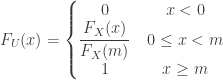


 and
and  . Thus the distribution function
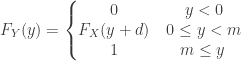
 and
and 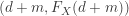 leftward to the point
  .
.![P[X<d]](https://s0.wp.com/latex.php?latex=P%5BX%3Cd%5D&bg=ffffff&fg=333333&s=-1&c=20201002) and the point mass at
and the point mass at ![P[X \ge d+m]](https://s0.wp.com/latex.php?latex=P%5BX+%5Cge+d%2Bm%5D&bg=ffffff&fg=333333&s=-1&c=20201002) . Thus the following is the density function of the “per loss” insurance payout
. Thus the following is the density function of the “per loss” insurance payout 
![\displaystyle E[Y]=\int_0^m y \thinspace f_X(y+d) \thinspace dy + m \thinspace [1-F_X(d+m)]](https://s0.wp.com/latex.php?latex=%5Cdisplaystyle+E%5BY%5D%3D%5Cint_0%5Em+y+%5Cthinspace+f_X%28y%2Bd%29+%5Cthinspace+dy+%2B+m+%5Cthinspace+%5B1-F_X%28d%2Bm%29%5D&bg=ffffff&fg=333333&s=-1&c=20201002)
![\displaystyle E[Y^n]=\int_0^m y^n \thinspace f_X(y+d) \thinspace dy + m^n \thinspace [1-F_X(d+m)]](https://s0.wp.com/latex.php?latex=%5Cdisplaystyle+E%5BY%5En%5D%3D%5Cint_0%5Em+y%5En+%5Cthinspace+f_X%28y%2Bd%29+%5Cthinspace+dy+%2B+m%5En+%5Cthinspace+%5B1-F_X%28d%2Bm%29%5D&bg=ffffff&fg=333333&s=-1&c=20201002) for all integer
for all integer 
 be the payout for an insurance contract with the same policy maximum
 ![E[Y]](https://s0.wp.com/latex.php?latex=E%5BY%5D&bg=ffffff&fg=333333&s=-1&c=20201002) and
and ![E[Z]](https://s0.wp.com/latex.php?latex=E%5BZ%5D&bg=ffffff&fg=333333&s=-1&c=20201002) and
and ![E[Z^2]](https://s0.wp.com/latex.php?latex=E%5BZ%5E2%5D&bg=ffffff&fg=333333&s=-1&c=20201002) (see
(see ![\displaystyle E[Y]=\int_0^m y \thinspace \lambda e^{-\lambda (y+d)} \thinspace dy + m \thinspace [e^{-\lambda (d+m)}]](https://s0.wp.com/latex.php?latex=%5Cdisplaystyle+E%5BY%5D%3D%5Cint_0%5Em+y+%5Cthinspace+%5Clambda+e%5E%7B-%5Clambda+%28y%2Bd%29%7D+%5Cthinspace+dy+%2B+m+%5Cthinspace+%5Be%5E%7B-%5Clambda+%28d%2Bm%29%7D%5D&bg=ffffff&fg=333333&s=-1&c=20201002)
![\displaystyle =e^{-\lambda d} \thinspace \biggl(\int_0^m y \thinspace \lambda \thinspace e^{-\lambda y} \thinspace dy+m \thinspace e^{-\lambda m}\biggr)=e^{-\lambda d} E[Z]](https://s0.wp.com/latex.php?latex=%5Cdisplaystyle+%3De%5E%7B-%5Clambda+d%7D+%5Cthinspace+%5Cbiggl%28%5Cint_0%5Em+y+%5Cthinspace+%5Clambda+%5Cthinspace+e%5E%7B-%5Clambda+y%7D+%5Cthinspace+dy%2Bm+%5Cthinspace+e%5E%7B-%5Clambda+m%7D%5Cbiggr%29%3De%5E%7B-%5Clambda+d%7D+E%5BZ%5D&bg=ffffff&fg=333333&s=-1&c=20201002)
![\displaystyle E[Y^2]=\int_0^m y^2 \thinspace \lambda \thinspace e^{-\lambda (y+d)} \thinspace dy+m^2 \thinspace e^{-\lambda (d+m)}](https://s0.wp.com/latex.php?latex=%5Cdisplaystyle+E%5BY%5E2%5D%3D%5Cint_0%5Em+y%5E2+%5Cthinspace+%5Clambda+%5Cthinspace+e%5E%7B-%5Clambda+%28y%2Bd%29%7D+%5Cthinspace+dy%2Bm%5E2+%5Cthinspace+e%5E%7B-%5Clambda+%28d%2Bm%29%7D&bg=ffffff&fg=333333&s=-1&c=20201002)
![\displaystyle =e^{-\lambda d} \thinspace \biggl(\int_0^m y^2 \thinspace \lambda \thinspace e^{-\lambda y} \thinspace dy+m^2 \thinspace e^{-\lambda m}\biggr)=e^{-\lambda d} E[Z^2]](https://s0.wp.com/latex.php?latex=%5Cdisplaystyle+%3De%5E%7B-%5Clambda+d%7D+%5Cthinspace+%5Cbiggl%28%5Cint_0%5Em+y%5E2+%5Cthinspace+%5Clambda+%5Cthinspace+e%5E%7B-%5Clambda+y%7D+%5Cthinspace+dy%2Bm%5E2+%5Cthinspace+e%5E%7B-%5Clambda+m%7D%5Cbiggr%29%3De%5E%7B-%5Clambda+d%7D+E%5BZ%5E2%5D&bg=ffffff&fg=333333&s=-1&c=20201002)
![\displaystyle Var[Y]=e^{-\lambda d} E[Z^2] - e^{-2 \lambda d} E[Z]^2](https://s0.wp.com/latex.php?latex=%5Cdisplaystyle+Var%5BY%5D%3De%5E%7B-%5Clambda+d%7D+E%5BZ%5E2%5D+-+e%5E%7B-2+%5Clambda+d%7D+E%5BZ%5D%5E2&bg=ffffff&fg=333333&s=-1&c=20201002)
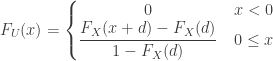
 . With the addition of a deductible
  . The expected insurance payout is reduced by the amount
 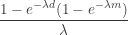 . Then the fraction of the loss eliminated by the deductible and the policy cap is
  . Note that the fraction of the loss eliminated by the policy cap alone is
  .
.
![Var[Z]](https://s0.wp.com/latex.php?latex=Var%5BZ%5D&bg=ffffff&fg=333333&s=-1&c=20201002) , that is when there is a deductible on top of the policy maximum, the variance of the “per loss” payout is less than the variance when there is only a policy maximum. We have the following derivation and the following claim:
, that is when there is a deductible on top of the policy maximum, the variance of the “per loss” payout is less than the variance when there is only a policy maximum. We have the following derivation and the following claim:![\displaystyle =e^{-\lambda d} (Var[Z]+E[Z]^2) - e^{-2 \lambda d} E[Z]^2](https://s0.wp.com/latex.php?latex=%5Cdisplaystyle+%3De%5E%7B-%5Clambda+d%7D+%28Var%5BZ%5D%2BE%5BZ%5D%5E2%29+-+e%5E%7B-2+%5Clambda+d%7D+E%5BZ%5D%5E2&bg=ffffff&fg=333333&s=-1&c=20201002)
![\displaystyle =e^{-\lambda d} Var[Z] + (e^{-\lambda d}-e^{-2 \lambda d}) E[Z]^2](https://s0.wp.com/latex.php?latex=%5Cdisplaystyle+%3De%5E%7B-%5Clambda+d%7D+Var%5BZ%5D+%2B+%28e%5E%7B-%5Clambda+d%7D-e%5E%7B-2+%5Clambda+d%7D%29+E%5BZ%5D%5E2&bg=ffffff&fg=333333&s=-1&c=20201002)
![\displaystyle Var[Z]>e^{-\lambda d} Var[Z] + (e^{-\lambda d}-e^{-2 \lambda d}) E[Z]^2](https://s0.wp.com/latex.php?latex=%5Cdisplaystyle+Var%5BZ%5D%3Ee%5E%7B-%5Clambda+d%7D+Var%5BZ%5D+%2B+%28e%5E%7B-%5Clambda+d%7D-e%5E%7B-2+%5Clambda+d%7D%29+E%5BZ%5D%5E2&bg=ffffff&fg=333333&s=-1&c=20201002)
![\displaystyle Var[Z] \le e^{-\lambda d} Var[Z] + (e^{-\lambda d}-e^{-2 \lambda d}) E[Z]^2](https://s0.wp.com/latex.php?latex=%5Cdisplaystyle+Var%5BZ%5D+%5Cle+e%5E%7B-%5Clambda+d%7D+Var%5BZ%5D+%2B+%28e%5E%7B-%5Clambda+d%7D-e%5E%7B-2+%5Clambda+d%7D%29+E%5BZ%5D%5E2&bg=ffffff&fg=333333&s=-1&c=20201002)
![\displaystyle (1-e^{-\lambda d}) Var[Z] \le e^{-\lambda d}(1-e^{-\lambda d})E[Z]^2](https://s0.wp.com/latex.php?latex=%5Cdisplaystyle+%281-e%5E%7B-%5Clambda+d%7D%29+Var%5BZ%5D+%5Cle+e%5E%7B-%5Clambda+d%7D%281-e%5E%7B-%5Clambda+d%7D%29E%5BZ%5D%5E2&bg=ffffff&fg=333333&s=-1&c=20201002)
![\displaystyle Var[Z] \le e^{-\lambda d}E[Z]^2](https://s0.wp.com/latex.php?latex=%5Cdisplaystyle+Var%5BZ%5D+%5Cle+e%5E%7B-%5Clambda+d%7DE%5BZ%5D%5E2&bg=ffffff&fg=333333&s=-1&c=20201002)
 . Thus
 ![Var[Z] \le 0](https://s0.wp.com/latex.php?latex=Var%5BZ%5D+%5Cle+0&bg=ffffff&fg=333333&s=-1&c=20201002) . This is a contradiction as
. This is a contradiction as ![Var[Z]>0](https://s0.wp.com/latex.php?latex=Var%5BZ%5D%3E0&bg=ffffff&fg=333333&s=-1&c=20201002) . Thus
. Thus  . This type of insurance contracts is also called the excess-of-loss contracts, since the insurer agrees to pay the insured the amount of the random loss
 . The following is the distribution function of

![\displaystyle E[Y]=\int_o^{\infty} y \thinspace f_X(y+d) \thinspace dy](https://s0.wp.com/latex.php?latex=%5Cdisplaystyle+E%5BY%5D%3D%5Cint_o%5E%7B%5Cinfty%7D+y+%5Cthinspace+f_X%28y%2Bd%29+%5Cthinspace+dy&bg=ffffff&fg=333333&s=-1&c=20201002)
![\displaystyle E[Y^n]=\int_o^{\infty} y^n \thinspace f_X(y+d) \thinspace dy](https://s0.wp.com/latex.php?latex=%5Cdisplaystyle+E%5BY%5En%5D%3D%5Cint_o%5E%7B%5Cinfty%7D+y%5En+%5Cthinspace+f_X%28y%2Bd%29+%5Cthinspace+dy&bg=ffffff&fg=333333&s=-1&c=20201002) for all integer
for all integer 
 . As a result, the density of the insurance payout is:
![\displaystyle E[Y]=\int_o^{\infty} y \thinspace \lambda e^{-\lambda (y+d)} \thinspace dy=\frac{e^{-\lambda d}}{\lambda}](https://s0.wp.com/latex.php?latex=%5Cdisplaystyle+E%5BY%5D%3D%5Cint_o%5E%7B%5Cinfty%7D+y+%5Cthinspace+%5Clambda+e%5E%7B-%5Clambda+%28y%2Bd%29%7D+%5Cthinspace+dy%3D%5Cfrac%7Be%5E%7B-%5Clambda+d%7D%7D%7B%5Clambda%7D&bg=ffffff&fg=333333&s=-1&c=20201002)
![\displaystyle E[Y^2]=\int_o^{\infty} y^2 \thinspace \lambda e^{-\lambda (y+d)} \thinspace dy=\frac{2 e^{- \lambda d}}{\lambda^2}](https://s0.wp.com/latex.php?latex=%5Cdisplaystyle+E%5BY%5E2%5D%3D%5Cint_o%5E%7B%5Cinfty%7D+y%5E2+%5Cthinspace+%5Clambda+e%5E%7B-%5Clambda+%28y%2Bd%29%7D+%5Cthinspace+dy%3D%5Cfrac%7B2+e%5E%7B-+%5Clambda+d%7D%7D%7B%5Clambda%5E2%7D&bg=ffffff&fg=333333&s=-1&c=20201002)
![\displaystyle Var[Y]=\frac{2 e^{- \lambda d}}{\lambda^2}-\biggl(\frac{e^{-\lambda d}}{\lambda}\biggr)^2=\frac{1}{\lambda^2} \thinspace e^{-\lambda d} \thinspace (2-e^{-\lambda d})](https://s0.wp.com/latex.php?latex=%5Cdisplaystyle+Var%5BY%5D%3D%5Cfrac%7B2+e%5E%7B-+%5Clambda+d%7D%7D%7B%5Clambda%5E2%7D-%5Cbiggl%28%5Cfrac%7Be%5E%7B-%5Clambda+d%7D%7D%7B%5Clambda%7D%5Cbiggr%29%5E2%3D%5Cfrac%7B1%7D%7B%5Clambda%5E2%7D+%5Cthinspace+e%5E%7B-%5Clambda+d%7D+%5Cthinspace+%282-e%5E%7B-%5Clambda+d%7D%29&bg=ffffff&fg=333333&s=-1&c=20201002)
 . Due to the ductible, the “per loss” payout is reduced by the amount
  . The fraction of the expected loss eliminated by the presence of the deductible is
 ![Var[Y] < \frac{1}{\lambda^2}](https://s0.wp.com/latex.php?latex=Var%5BY%5D+%3C+%5Cfrac%7B1%7D%7B%5Clambda%5E2%7D&bg=ffffff&fg=333333&s=-1&c=20201002) .
.