In this post, we discuss the compound negative binomial distribution and its relationship with the compound Poisson distribution.
A compound distribution is a model for a random sum  where the number of terms
  is uncertain. To make the compund distribution more tractable, we assume that the variables
  are independent and identically distributed and that each is independent of . The random sum
  can be interpreted the sum of all the measurements that are associated with certain events that occur during a fixed period of time. For example, we may be interested in the total amount of rainfall in a 24-hour period, during which the occurences of a number of events are observed and each of the events provides a measurement of an amount of rainfall. Another interpretation of compound distribution is the random variable of the aggregate claims generated by an insurance policy or a group of insurance policies during a fixed policy period. In this setting, is the number of claims generated by the portfolio of insurance policies and
  is the amount of the first claim and
  is the amount of the second claim and so on. When follows the Poisson distribution, the random sum is said to have a compound Poisson distribution. Even though the compound Poisson distribution has many attractive properties, it is not a good model when the variance of the number of claims is greater than the mean of the number of claims. In such situations, the compound negative binomial distribution may be a better fit. See this post (Compound Poisson distribution) for a basic discussion. See the links at the end of this post for more articles on compound distributons that I posted on this blog.
Compound Negative Binomial Distribution
The random variable is said to have a negative binomial distribution if its probability function is given by the following:
![\displaystyle P[N=n]=\binom{\alpha + n-1}{\alpha-1} \thinspace \biggl(\frac{\beta}{\beta+1}\biggr)^{\alpha}\biggl(\frac{1}{\beta+1}\biggr)^{n} \ \ \ \ \ \ \ \ \ \ \ \ (1)](https://s0.wp.com/latex.php?latex=%5Cdisplaystyle+P%5BN%3Dn%5D%3D%5Cbinom%7B%5Calpha+%2B+n-1%7D%7B%5Calpha-1%7D+%5Cthinspace+%5Cbiggl%28%5Cfrac%7B%5Cbeta%7D%7B%5Cbeta%2B1%7D%5Cbiggr%29%5E%7B%5Calpha%7D%5Cbiggl%28%5Cfrac%7B1%7D%7B%5Cbeta%2B1%7D%5Cbiggr%29%5E%7Bn%7D+%5C+%5C+%5C+%5C+%5C+%5C+%5C+%5C+%5C+%5C+%5C+%5C+%281%29&bg=ffffff&fg=333333&s=-1&c=20201002)
where 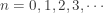 ,
,  and
and  is a positive integer.
Our formulation of negative binomial distribution is the number of failures that occur before the  success in a sequence of independent Bernoulli trials. But this interpretation is not important to our task at hand. Let be the random sum as described in the above introductory paragraph such that follows a negative binomial distribution. We present the basic properties discussed in the post An introduction to compound distributions by plugging the negative binomial distribution into .
Distribution Function
![\displaystyle F_Y(y)=\sum \limits_{n=0}^{\infty} F^{*n}(y) \thinspace P[N=n]](https://s0.wp.com/latex.php?latex=%5Cdisplaystyle+F_Y%28y%29%3D%5Csum+%5Climits_%7Bn%3D0%7D%5E%7B%5Cinfty%7D+F%5E%7B%2An%7D%28y%29+%5Cthinspace+P%5BN%3Dn%5D&bg=ffffff&fg=333333&s=-1&c=20201002)
where  is the common distribution function for and
  is the
  convolution of . Of course,
 ![P[N=n]](https://s0.wp.com/latex.php?latex=P%5BN%3Dn%5D&bg=ffffff&fg=333333&s=-1&c=20201002) is the negative binomial probability function indicated above.
is the negative binomial probability function indicated above.
Mean and Variance
![\displaystyle E[Y]=E[N] \thinspace E[X]=\frac{\alpha}{\beta} E[X]](https://s0.wp.com/latex.php?latex=%5Cdisplaystyle+E%5BY%5D%3DE%5BN%5D+%5Cthinspace+E%5BX%5D%3D%5Cfrac%7B%5Calpha%7D%7B%5Cbeta%7D+E%5BX%5D&bg=ffffff&fg=333333&s=-1&c=20201002)
![\displaystyle Var[Y]=E[N] \thinspace Var[X]+Var[N] \thinspace E[X]^2](https://s0.wp.com/latex.php?latex=%5Cdisplaystyle+Var%5BY%5D%3DE%5BN%5D+%5Cthinspace+Var%5BX%5D%2BVar%5BN%5D+%5Cthinspace+E%5BX%5D%5E2&bg=ffffff&fg=333333&s=-1&c=20201002)
![\displaystyle =\frac{\alpha}{\beta} Var[X]+\frac{\alpha (\beta+1)}{\beta^2} E[X]^2](https://s0.wp.com/latex.php?latex=%5Cdisplaystyle+%3D%5Cfrac%7B%5Calpha%7D%7B%5Cbeta%7D+Var%5BX%5D%2B%5Cfrac%7B%5Calpha+%28%5Cbeta%2B1%29%7D%7B%5Cbeta%5E2%7D+E%5BX%5D%5E2&bg=ffffff&fg=333333&s=-1&c=20201002)
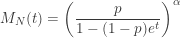
Moment Generating Function
![\displaystyle M_Y(t)=M_N[ln M_X(t)]=\biggl(\frac{p}{1-(1-p) M_X(t)}\biggr)^{\alpha}](https://s0.wp.com/latex.php?latex=%5Cdisplaystyle+M_Y%28t%29%3DM_N%5Bln+M_X%28t%29%5D%3D%5Cbiggl%28%5Cfrac%7Bp%7D%7B1-%281-p%29+M_X%28t%29%7D%5Cbiggr%29%5E%7B%5Calpha%7D&bg=ffffff&fg=333333&s=-1&c=20201002)

where  ,
, 
Cumulant Generating Function
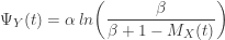
Skewness
![\displaystyle E[(Y-\mu_Y)^3]=\Psi_Y^{(3)}(0)](https://s0.wp.com/latex.php?latex=%5Cdisplaystyle+E%5B%28Y-%5Cmu_Y%29%5E3%5D%3D%5CPsi_Y%5E%7B%283%29%7D%280%29&bg=ffffff&fg=333333&s=-1&c=20201002)
![\displaystyle =\frac{2}{\alpha^2} E[N]^3 E[X]^3 +\frac{3}{\alpha} E[N]^2 E[X] E[X^2]+E[N] E[X^3]](https://s0.wp.com/latex.php?latex=%5Cdisplaystyle+%3D%5Cfrac%7B2%7D%7B%5Calpha%5E2%7D+E%5BN%5D%5E3+E%5BX%5D%5E3+%2B%5Cfrac%7B3%7D%7B%5Calpha%7D+E%5BN%5D%5E2+E%5BX%5D+E%5BX%5E2%5D%2BE%5BN%5D+E%5BX%5E3%5D&bg=ffffff&fg=333333&s=-1&c=20201002)
Measure of skewness: ![\displaystyle \gamma_Y=\frac{E[(Y-\mu_Y)^3]}{(Var[Y])^{\frac{3}{2}}}](https://s0.wp.com/latex.php?latex=%5Cdisplaystyle+%5Cgamma_Y%3D%5Cfrac%7BE%5B%28Y-%5Cmu_Y%29%5E3%5D%7D%7B%28Var%5BY%5D%29%5E%7B%5Cfrac%7B3%7D%7B2%7D%7D%7D&bg=ffffff&fg=333333&s=-1&c=20201002)
Compound Mixed Poisson Distribution
In a previous post (Basic properties of mixtures), we showed that the negative binomial distribution is a mixture of a family of Poisson distributions with gamma mixing weights. Specifically, if 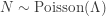 and
and  , then the unconditional distribution of is a negative binomial distribution and the probability function is of the form (1) given above.
Thus the negative binomial distribution is a special example of a compound mixed Poisson distribution. When an aggregate claims variable  has a compound mixed Poisson distribution, the number of claims follows a Poisson distribution, but the Poisson parameter
  is uncertain. The uncertainty could be due to an heterogeneity of risks across the insureds in the insurance portfolio (or across various rating classes). If the information of the risk parameter can be captured in a gamma distribution, then the unconditional number of claims in a given fixed period has a negative binomial distribution.
Previous Posts on Compound Distributions
An introduction to compound distributions
Some examples of compound distributions
Compound Poisson distribution
Compound Poisson distribution-discrete example

